This post is part 3 of the "Approximating Skills of Table Tennis Players Using Normal Distribution" series:
- Approximating Skills of Table Tennis Players Using Normal Distribution. Introduction
- Mathematical Model for Player Ranking
- Fitting the Player Ranking Model: A Maximum Likelihood Approach
In the previous post, we built all the necessary mathematics to model player skills as normal distributions. Here we will use all the formulas to implement the optimization algorithm in Python and fit the model to the data (both synthetic and real).
General setup
We will code everything from scratch - this will help us understand the mathematics better and give us more flexibility and fine-grained control over the model.
As for libraries, we will use only numpy and scipy for numerical computations and access to the norm
distribution. And, of course, matplotlib for plotting.
import matplotlib.pyplot as plt
import numpy as np
from scipy.stats import norm
Optimization algorithm
The algorithm will be an exact copy of what we derived in the previous post. We will start with the optimization function itself, and then implement all the necessary helper functions. We will initialize means and scales (\(\theta\)) with zeros for means and ones for scales, and then use gradient ascent to optimize them.
def optimize(
        n_players: int,
        dataset: np.ndarray,
        alpha: float = 1e-4,
        epochs: int = 1000,
        logger: Logger | None = None,
) -> np.ndarray:
    # setting theta to an arbitrary value - mean 0 and scale 1 for each player
    theta = np.full((n_players, 2), [0.0, 1.0])

    iteration = 1
    while iteration <= epochs:
        # calculating gradients of log likelihood
        grads = grad_log_likelihood(theta, dataset)

        # updating theta
        theta += alpha * grads

        # calculating likelihood
        likelihood = log_likelihood(theta, dataset)

        # log iteration values
        if logger:
            logger.log('log_likelihood', likelihood.mean(), iteration)
            logger.log('grad_norm', np.linalg.norm(grads), iteration)

        # incrementing iteration
        iteration += 1
    return theta
The primary optimize function that performs all the training using gradient ascent.
What’s happening here:
n_players: number of players participating in the tournament; we can’t rely on the dataset to tell us this, as it may contain only a subset of players. We won’t be able to calculate the means and scales for these “missing” players, obviously, but we will still need to initialize them.dataset: a 2D array of shape(n_games, 2)containing game outcomes, where each row is a game with two players - the first player won, and the second lost.alpha: learning rate for the gradient ascent; we will use a small value to ensure smooth convergence.epochs: number of iterations to run the optimization; we will stop when we reach this number.logger: it’s really useful to log the optimization process; we will use it to track the progress and visualize the results. Everybody loves a good smooth plot.theta: a 2D array of shape(n_players, 2)containing means and scales for each player; we will optimize these values during the training process. We initialize it with zeros for means and ones for scales.grads: gradients of the log likelihood function.likelihood: value of the log likelihood function for the current iteration - we’ll plot it later to see how the optimization process goes.
Not rocket science, actually. Let’s start with the log_likelihood function - it’s a bit easier than the gradient one.
However, we’ll still need a couple more helper functions to calculate the probabilities of winning and losing,
specifically, the CDF and PDF of the standard normal distribution. Fortunately, scipy.stats.norm has it all.
def norm_diff_argument(theta: np.ndarray, dataset: np.ndarray) -> np.ndarray:
    # returns - (mu1 - mu2) / sqrt(sigma1^2 + sigma2^2) for each game in the dataset
    means = theta[:, 0]
    scales = theta[:, 1]
    winners = dataset[:, 0]
    losers = dataset[:, 1]
    return -(means[winners] - means[losers]) / np.sqrt(scales[winners] ** 2 + scales[losers] ** 2)


def Phi(x: np.ndarray) -> np.ndarray:
    # returns the Cumulative Distribution Function of the standard normal distribution at the given point
    return norm.cdf(x, loc=0, scale=1)


def phi(x: np.ndarray) -> np.ndarray:
    # returns the Probability Density Function of the standard normal distribution at the given point
    return norm.pdf(x, loc=0, scale=1)
Now, from the mathematical model, we know how to calculate the log likelihood of the dataset given the parameters:
We will return not a sum, but all the values in a 1D array.
def log_likelihood(theta: np.ndarray, dataset: np.ndarray) -> np.ndarray:
    x = norm_diff_argument(theta, dataset)
    return np.log(1 - Phi(x))
The log_likelihood function that calculates the log likelihood of the games dataset given the parameters \(\theta\).
Okay, now to the most interesting part - the gradient of the log likelihood function. We will leverage numpy vectorization to perform the calculations efficiently - without any loops. It’s a bit tricky and requires some “thinking”, but it’s much easier to read the code, and it’ll also be much more concise and faster than the naive implementation.
Besides, as we see in the gradient formula, there are a couple of things that we can precompute for both means and scales gradients. First, we will precompute the common term
Second, to calculate the gradients for each player, we will need to find all the games where the player either won or
lost. We will mark games with 0 if the player didn’t participate, 1 if the player won, and -1 if the player lost.
def grad_log_likelihood(theta: np.ndarray, dataset: np.ndarray) -> np.ndarray:
    players = np.arange(theta.shape[0]).reshape(-1, 1)
    scales = theta[:, 1]
    winners = dataset[:, 0]
    losers = dataset[:, 1]

    x = norm_diff_argument(theta, dataset)

    # common multipliers for both gradients
    phi_by_one_minus_Phi = phi(x) / (1 - Phi(x))

    # -1/0/1 matrix indicating which player is winner/none/loser in each game
    players_x_games = (players == winners).astype(int) - (players == losers).astype(int)

    # calculating gradients for means
    means_grad = players_x_games @ (phi_by_one_minus_Phi / np.sqrt(scales[winners] ** 2 + scales[losers] ** 2))

    # calculating gradients for scales
    scales_grad = np.abs(players_x_games) @ (phi_by_one_minus_Phi * x / (scales[winners] ** 2 + scales[losers] ** 2)) * scales

    # returning gradients as a concatenated array in the form of theta
    return np.vstack([means_grad, scales_grad]).transpose()
The grad_log_likelihood function that calculates the gradient of the log likelihood function for the games dataset.
That’s pretty much it, and we’re ready to test our implementation!
Testing the implementation
We will start with a synthetic dataset - a sanity check to ensure that all the mathematics and implementation are correct. We will attribute the players with random means and scales, and then generate a random dataset with game outcomes based on these parameters. So ideally we should be able to recover the original means and scales from the dataset (or at least end up with values that will produce the same probabilities of winning and losing for player pairs).
I’ll also include here a couple of utility functions to generate the dataset, plot the results, print metrics, as well as the main function to run the optimization.
class Logger:
    def __init__(self):
        self._metrics = {}

    def log(self, metric: str, value: float, iteration: int):
        if metric not in self._metrics:
            self._metrics[metric] = {}
        self._metrics[metric][iteration] = value


def plot(
        *args,
        diagram = plt.plot,
        label: str = None,
        xlabel: str = None,
        ylabel: str = None,
        title: str = None,
        **kwargs
):
    plt.figure(figsize=(10, 5))
    diagram(*args, label=label, **kwargs)
    plt.xlabel(xlabel)
    plt.ylabel(ylabel)
    plt.title(title)
    plt.legend()
    plt.savefig(label.replace(' ', '_').lower() + '.png')


def print_metrics(theta: np.ndarray, optimized_theta: np.ndarray):
    print(f'Initial means: {theta[:, 0]}')
    print(f'Optimized means: {optimized_theta[:, 0]}')
    print(f'Initial scales: {theta[:, 1]}')
    print(f'Optimized scales: {optimized_theta[:, 1]}')

    p_diff = []
    for p1 in range(theta.shape[0] - 1):
        for p2 in range(p1 + 1, theta.shape[0]):
            p_real = 1 - Phi(-(theta[p1, 0] - theta[p2, 0]) / np.sqrt(theta[p1, 1] ** 2 + theta[p2, 1] ** 2))
            p_optimized = 1 - Phi(-(optimized_theta[p1, 0] - optimized_theta[p2, 0]) / np.sqrt(optimized_theta[p1, 1] ** 2 + optimized_theta[p2, 1] ** 2))
            p_diff.append(p_real - p_optimized)

    print(f'Mean difference in probabilities: {np.mean(np.abs(p_diff)):.4f}')
    print(f'Median difference in probabilities: {np.median(np.abs(p_diff)):.4f}')

    plot(
        p_diff,
        diagram=plt.hist,
        bins=10,
        alpha=0.7,
        label='Probability Differences',
        xlabel='Probability Difference',
        ylabel='Value',
        title='Distribution of Probability Differences'
    )


def generate_games(means: np.ndarray, scales: np.ndarray, n_games: int) -> np.ndarray:
    winners = []
    losers = []
    # creating an array of players indices
    players = np.arange(means.size)
    for i in range(n_games):
        # taking 2 players at random
        ps = np.random.choice(players, 2, False)
        # generating skills for these players using normal distribution
        skills = np.random.normal(loc=means[ps], scale=scales[ps])
        # winner is the player with higher skill, loser is the one with lower skill
        winners.append(ps[np.argmax(skills)])
        losers.append(ps[np.argmin(skills)])
    return np.vstack([winners, losers]).transpose()


if __name__ == '__main__':
    # Example usage
    n_players = 10
    n_games = 300

    # Randomly generating means and scales for players
    means = np.random.uniform(0, 5, n_players)
    scales = np.random.uniform(0.5, 2, n_players)

    # Generating games dataset
    games_dataset = generate_games(means, scales, n_games)

    # Initializing logger
    logger = Logger()

    # Optimizing player skills
    optimized_theta = optimize(n_players, games_dataset, alpha=1e-4, epochs=5000, logger=logger)

    # Printing results
    print_metrics(np.vstack([means, scales]).transpose(), optimized_theta)

    # plotting the results for visualization of logs - saving into a file
    plot(
        list(logger._metrics['log_likelihood'].keys()),
        list(logger._metrics['log_likelihood'].values()),
        label='Log Likelihood',
        xlabel='Iteration',
        ylabel='Value',
        title='Log Likelihood Over Iterations'
    )
    plot(
        list(logger._metrics['grad_norm'].keys()),
        list(logger._metrics['grad_norm'].values()),
        label='Gradient Norm',
        xlabel='Iteration',
        ylabel='Value',
        title='Gradient Norm Over Iterations'
    )
Note: It is an interesting question how to measure the difference between two probability distributions, since we want to compare the original and optimized distributions for each pair of players. There are many smart approaches to do so, e.g. Kullback-Leibler divergence, but I really prefer something simple, intuitive, and interpretable. So here I just calculate the absolute difference between the probabilities of winning for each pair of players, and then take the mean and median of these differences. Ideally, we should see that these differences are small, which means that the optimized parameters produce probabilities of winning and losing that are close to the original ones.
Cool! Now - the most interesting part - let’s see the results. Again, ideally we should see that:
- Log likelihood is increasing over iterations - it means that the model is learning and improving its fit to the data.
- Gradient norm is decreasing over iterations - it means that the model is converging to an optimal (or suboptimal) solution.
- The optimized means and scales produce probabilities of winning and losing that are close to the original ones - it means that the model is able to recover the original interconnections between players’ skills and game outcomes.
Here is the output:
Initial means: [3.84361067 3.83766923 2.67264325 4.11026263 0.6825908  1.50171865 2.20568889 0.53084076 0.40802729 1.36410144]
Optimized means: [ 0.90024205  0.91925092  0.34922694  0.95610695 -0.66441085 -0.17676143 -0.1826733  -0.7631907  -1.10177428 -0.23601631]
Initial scales: [0.6120189  0.88244972 1.9428094  1.2859601  1.37018517 1.52210234 1.26951214 1.80880291 1.90045287 1.60969589]
Optimized scales: [0.87155517 0.5327172  0.3682235  0.5299672  0.819666   0.59379071 0.47543815 0.61261271 0.94202693 0.99237121]
Mean difference in probabilities: 0.0618
Median difference in probabilities: 0.0524
We can see that the optimized means and scales are quite different from the original ones, but the probabilities of
winning and losing for each pair of players are still close to the original ones. The mean difference is around 0.06,
which means that when predicting the outcome of a game between two players, the model will be off by about 6% on
average. Looks nice, actually!
What about the plots?
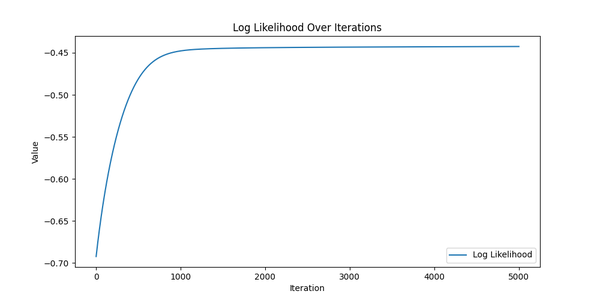
Log Likelihood over iterations.
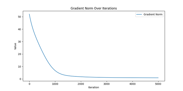
Gradient Norm over iterations.
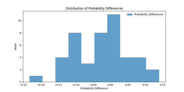
Distribution of Probability Differences.
They look like we actually trained something! All charts show exactly what we expected: the log likelihood is increasing, the gradient norm is decreasing, and the probability differences are distributed around zero with small variation. So it looks like we’re ready to move on to the real data.
However, just out of curiosity, let’s compare log likelihoods for the original and optimized parameters.
Log likelihood - initial   : -0.4194
Log likelihood - optimized : -0.4403
They are roughly the same, which means that the model is able to fit the data well enough. We’re good to go!
Applying the model to real data
There were 11 participants in the tournament, and we had to play one against each other to determine the ranking (since I started this project after the tournament). We played “until 2 wins” in a best-of-3 format, and the final table looks like this:
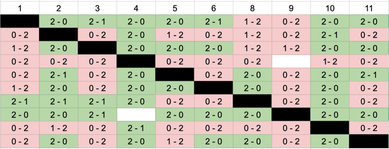
The final table of the tournament.
Anyway, we have the data, and we can use it to fit our model. I’ll omit the data transformation part here, and run the
optimize function to see what we get. Let’s start with the plots:
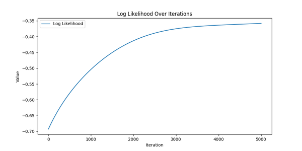
Log Likelihood over iterations for real data.
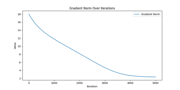
Gradient Norm over iterations for real data.
The same picture as before: the log likelihood is increasing, the gradient norm is decreasing; looks like it converged. But now, contrary to the synthetic data, we don’t have the “original” means and scales to compare with. So let’s compare the optimized means and scales with some basic statistics of the players’ performance like the number of wins/losses (side note: some players played more games than others due to “finals” and absences).
| Player | # wins | # losses | Skill mean | Skill variance |
|---|---|---|---|---|
| 1 | 7 | 2 | 0.77 | 0.55 |
| 2 | 2 | 7 | -0.66 | 0.42 |
| 3 | 8 | 3 | 0.98 | 0.31 |
| 4 | 0 | 8 | -1.52 | 0.33 |
| 5 | 5 | 4 | -0.03 | 0.45 |
| 6 | 5 | 4 | 0.24 | 0.19 |
| 7 | 5 | 4 | 0.01 | 1.17 |
| 8 | 9 | 1 | 1.12 | 0.55 |
| 9 | 1 | 8 | -1.18 | 0.45 |
| 10 | 5 | 6 | 0.29 | 0.32 |
Looks somewhat close to what we expected - the players with more wins have higher means. The scales are a bit more tricky, but they also seem to reflect the players’ performance - those with an almost equal number of wins and losses have higher scales, while those with a clear advantage have lower scales.
Back then we also calculated the final ranking manually, based on the number of wins and losses. Let’s compare it with the ranking based on the optimized means. A couple of notes here: first, we had “finals” among the top three players at the end, and second, player #1 didn’t participate in the finals due to an injury, so we had to adjust the final ranking.
| Player | Manual ranking before finals | Manual ranking after finals | Skill ranking | Skill mean |
|---|---|---|---|---|
| 1 | 2 | 4 | 3 | 0.77 |
| 2 | 8 | 8 | 8 | -0.66 |
| 3 | 3 | 1 | 2 | 0.98 |
| 4 | 10 | 10 | 10 | -1.52 |
| 5 | 6 | 6 | 7 | -0.03 |
| 6 | 5 | 5 | 5 | 0.24 |
| 7 | 7 | 7 | 6 | 0.01 |
| 8 | 1 | 2 | 1 | 1.12 |
| 9 | 9 | 9 | 9 | -1.18 |
| 10 | 4 | 3 | 4 | 0.29 |
The ranking based on the optimized means is really close to the manual ranking! Which means that we could have used this model to determine the ranking without manual calculations (if only I had this model before the tournament).
However, the most useful part of this model is that it allows us to predict the outcome of future games between players. Here’s the table with the probabilities of winning for each player against each other player (the probability that the player on the left will win against the player on the top):
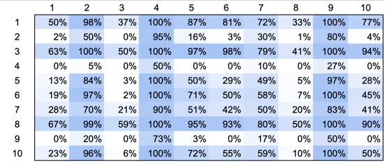
Winning probabilities for each player against each other.
Conclusion
This whole exercise was done just out of curiosity and for fun! But I also wanted to show how mathematics and programming can be used to solve real-world problems, and I hope you enjoyed it. Maybe it will even encourage you to try something similar on your own.
Full code is available on GitHub.