Mathematical Model for Player Ranking

This post is part 2 of the "Approximating Skills of Table Tennis Players Using Normal Distribution" series:

In the previous post, we discussed how to model player skills using normal distributions. Now, let’s dive into the mathematical details of how we can estimate the parameters of these distributions using Maximum Likelihood Estimation.

Problem definition: Having a set of players $\mathcal{P}$ numbered from $1$ to $n$ and a set of game results $\mathcal{D}$ assign skill levels to each player modeling it with normal distribution.

Definitions

First, let’s start with definitions and basic observations.

Set of players $\mathcal{P}$

There are $n$ players playing in a table tennis tournament. We’ll refer to the set of players as $\mathcal{P}$. For the sake of simplicity, we will assign a number between $1$ and $n$ to each player, essentially replacing players with the corresponding numbers in our model, so ${\mathcal{P}=\{1, 2, ..., n\}, |\mathcal{P}|=n}$.

Set of game results $\mathcal{D}$

First, there are no draws. Second, we don’t know the exact (or even approximate) skills of players. The only thing we know is who won in a single game between two players. So, each game can be modeled as a tuple ${(p_1, p_2), \;p_{1,2}\in\mathcal{P}}$, meaning that player $p_1$ won against player $p_2$.

Moreover, the same players may play against each other multiple times, and their games may even end with different outcomes. So the set of game results can look like

$$ \mathcal{D}=\{(1,2), (1, 2), (2, 1), (2, 3), (4, 2), ...\} $$

More formally,

\begin{equation} \mathcal{D}=\{G^k_{p_i, p_j}\;|\;p_i, p_j \in \mathcal{P}, \; k=\overline{1, m} \}, \; G^k_{p_i, p_j}=(p_i, p_j), \; |\mathcal{D}|=m \end{equation}

Calculating probability of a game outcome

Each player’s skill is drawn from their specific distribution $\mathcal{S}_i \sim \mathcal{N}(\mu_i,\,\sigma_i^2)\,$. The probability of an event $G_{p_i, p_j}=(p_i, p_j)$ where player $p_i$ wins against player $p_j$ can therefore be calculated as

\begin{equation} P(G_{p_i, p_j}) = P(S_{p_i}>S_{p_j})=P(S_{p_i}-S_{p_j}>0)=1 - P(S_{p_i}-S_{p_j}\leq 0) \end{equation}

Since $S_{p_i} \sim \mathcal{N}(\mu_{p_i},\,\sigma_{p_i}^2)\,$ and $S_{p_j} \sim \mathcal{N}(\mu_{p_j},\,\sigma_{p_j}^2)\,$, it’s quite easy to show that $Q_{p_ip_j} = S_{p_i}-S_{p_j}\sim \mathcal{N}({\mu_{p_i}-\mu_{p_j}},\,{\sigma_{p_i}^2+\sigma_{p_j}^2})\,$.

For standard normal distribution we know that

\begin{equation*} \begin{split} & z\sim\mathcal{N}(0,\,1)\, \implies P(z\leq 0)=F_z(0)=\Phi(0), \text{where} \\ & \Phi(x)=\frac{1}{\sqrt{2\pi}}\int_{-\infty}^{x}e^{-t^2/2}dt \end{split} \end{equation*}

Here $F_z(x)=P(z\leq x)$ is a Cumulative Distribution Function (CDF), and $\Phi(x)$ is how the CDF of the standard normal distribution is usually denoted. For general normal distribution we have

\begin{equation*} \begin{split} & \xi\sim\mathcal{N}(\mu,\,\sigma^2)\, \implies \xi = \sigma z + \mu \implies \\ & P(\xi\leq0)=F_{\xi}(0)=P(\sigma z + \mu \leq 0)=P\left(z \leq -\frac{\mu}{\sigma}\right) = F_z\left( -\frac{\mu}{\sigma} \right) = \Phi\left(-\frac{\mu}{\sigma}\right) \end{split} \end{equation*}

Together with the previous equation, it gives us

\begin{equation} \begin{split} & P(G_{p_i, p_j}) = 1 - P(S_{p_i}-S_{p_j}\leq0) = 1-P(Q_{p_ip_j} \leq 0) = \\ & = 1-F_{Q_{p_ip_j}}(0)=1-\Phi\left(-\frac{\mu_{p_i}-\mu_{p_j}}{\sqrt{\sigma_{p_i}^2+\sigma_{p_j}^2}}\right) \end{split} \end{equation}

Set of skills $\mathcal{S}$

With all mentioned above, we can say that $\mathcal{S}=\left\{ \mu_i \;|\; i = \overline{1, n} \right\}, \; |\mathcal{S}|= |\mathcal{P}| = n$, a set of mean skills of players. Finding $\mathcal{S}$ is essentially the goal of the whole process.

Maximum Likelihood Estimation

We will approach the problem with the Maximum Likelihood Estimation (MLE) method. There’s a lot of math behind it, but essentially it works as follows:

We have a set of observations, a dataset.
We want to model it with a certain statistical model, an approach
This model has a set of parameters that define the exact behavior of the model
We want to find these parameters, optimal values for them, so we can plug them into the model and make calculations and predictions
We do so by maximizing the probability of observing the given dataset, over all possible parameter values

How it all applies to our case:

It’s quite clear with the dataset of observations - that’s just the set of game outcomes, $\mathcal{D}$.
Statistical model: we say that in each game each player shows certain random skill drawn from their specific distribution, and wins against a player that showed lower skill, and that these distributions are modeled with normal distributions with different mean and scale values.
The set of parameters is, therefore, a set of mean/scale values, a total of $2n$ unknown parameters (since there are $n$ players in total). We can define it as
\begin{equation*} \theta= \begin{pmatrix} \mu_1 & \sigma_1\\ \mu_2 & \sigma_2\\ \vdots & \vdots\\ \mu_n & \sigma_n \end{pmatrix} \end{equation*}

The set of parameters $\theta$ is our target. We find it with MLE:

\begin{equation}\label{eq:mle} \mathcal{L}\left(\,\theta \; ; \; \mathcal{D} \,\right) = P_{\theta}\left(\,\mathcal{D} \,\right) \xrightarrow{\theta} \max \end{equation}

Here come a couple of simplifications: first, we assume that games are independent of each other, they are independent events; second, as mentioned before, each player’s distribution $\mathcal{S}_i$ is fixed, and not affected by other players. With that in mind, equations above give us the following:

\begin{equation} \begin{split} & \mathcal{L}\left(\,\theta \; ; \; \mathcal{D} \,\right) = P_{\theta}\left(\,\mathcal{D} \,\right) = P_\theta\left(\, G^0 \,G^1 \, \ldots G^m \,\right) = P_\theta\left(\, G^0 \,\right) \cdot P_\theta\left(\, G^1 \,\right) \cdot \ldots \cdot P_\theta\left(\, G^m \,\right) = \\ &= \prod_{i=1}^{m}{P_\theta\left(\, G^i \,\right) } = \prod_{i=1}^{m}{\left(1-P_\theta\left(\, S_{p_1^i} - S_{p_2^i} \leq 0 \,\right)\right)} =\\ &=\prod_{i=1}^{m}{\left(1-\Phi\left(-\frac{\mu_{\theta,\, p_1^i}-\mu_{\theta,\,p_2^i}}{\sqrt{\sigma_{\theta,\,p_1^i}^2+\sigma_{\theta,\,p_2^i}^2}}\right)\right)}\xrightarrow{\theta} \max \end{split} \end{equation}

There are different ways of finding the optimal (or sub-optimal) $\theta$ that maximizes MLE equation, but we’ll use a classic optimization approach widely used in machine learning — gradient descent (or ascent, depending on whether you strive for minimizing or maximizing a certain function). Its idea is quite simple:

We start with a random (or arbitrary) parameter set $\theta:=\theta_0$.
Then we calculate the gradient of the target function over the parameter set — $\nabla \mathcal{L}\left(\,\theta \; ; \; \mathcal{D} \,\right)$; it is the “direction” and the rate of the fastest increase at the point $\theta$. This direction is a vector, and has the same shape as $\theta$.
Finally, we update the current point $\theta$ slightly moving it towards the gradient direction (or opposite, depending on whether we’re looking for maximal or minimal value of the target function), and repeat the process until a certain stop criterion is reached (e.g., number of iterations).

Why do we do it slightly? Well, because we don’t want to overshoot the optima. A gradient in a certain point only gives us the direction and the rate of the fastest increase at that point. And gradients can change quite a lot as we move through the parameter space. So we take a small step in the gradient direction (or the opposite one), and then recalculate the gradient at the new point, and so on.

Gradient Descent

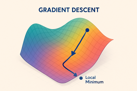
Gradient descent, as seen by ChatGPT

Calculating Gradients

Here will be a lot of math equations, so we’ll start with some notations and observations to make everything a bit easier to read. First, for standard normal distribution, we have:

\begin{equation*} \begin{split} & \phi(x) = \frac{1}{\sqrt{2\pi}}e^{-x^2/2} \; \text{ is a probability density function (PDF)} \\ & \Phi(x) = \int_{-\infty}^{x} \phi(t) dt \; \text{ is a cumulative distribution function (CDF)} \\ & \frac{\partial}{\partial x}\Phi(x) = \phi(x) \; \text{ is a derivative of the CDF} \\ & \frac{\partial}{\partial x} \Phi\left(f(x)\right) = \phi\left(f(x)\right) \cdot \frac{\partial f(x)}{\partial x} \; \text{ using a chain rule} \\ \end{split} \end{equation*}

Second, let’s recap that our target in MLE equation is to maximize the likelihood. But it’s the same as maximizing the logarithm of the likelihood (since logarithm is a monotonically increasing function), so we can take a logarithm of the whole equation and maximize it instead! This is a common practice in statistics, and it makes the math a bit easier.

\begin{equation} \begin{split} & \log{\mathcal{L}\left(\,\theta \; ; \; \mathcal{D} \,\right)} = \log{\prod_{i=1}^{m}{\left(1-\Phi\left(-\frac{\mu_{\theta,\, p_1^i}-\mu_{\theta,\,p_2^i}}{\sqrt{\sigma_{\theta,\,p_1^i}^2+\sigma_{\theta,\,p_2^i}^2}}\right)\right)}} = \\ & = \sum_{i=1}^{m}{\log{\left(1-\Phi\left(-\frac{\mu_{\theta,\, p_1^i}-\mu_{\theta,\,p_2^i}}{\sqrt{\sigma_{\theta,\,p_1^i}^2+\sigma_{\theta,\,p_2^i}^2}}\right)\right)}} \xrightarrow{\theta} \max \end{split} \end{equation}

To find the gradient of the log likelihood function, we need to differentiate it with respect to the parameters $\theta$. The gradient is a vector of partial derivatives of the log-likelihood function with respect to each parameter in $\theta$. As we have $2n$ parameters, we will have $2n$ partial derivatives; $n$ partial derivatives with respect to $\mu_i$ and $n$ partial derivatives with respect to $\sigma_i$:

\begin{equation} \nabla \log {\mathcal{L}\left(\,\theta \; ; \; \mathcal{D} \,\right)} = \begin{pmatrix} \frac{\partial \log {\mathcal{L}\left(\,\theta \; ; \; \mathcal{D} \,\right)}}{\partial \mu_1} & \frac{\partial \log {\mathcal{L}\left(\,\theta \; ; \; \mathcal{D} \,\right)}}{\partial \sigma_1}\\ \\ \frac{\partial \log {\mathcal{L}\left(\,\theta \; ; \; \mathcal{D} \,\right)}}{\partial \mu_2} & \frac{\partial \log {\mathcal{L}\left(\,\theta \; ; \; \mathcal{D} \,\right)}}{\partial \sigma_2}\\ \\ \vdots & \vdots\\ \\ \frac{\partial \log {\mathcal{L}\left(\,\theta \; ; \; \mathcal{D} \,\right)}}{\partial \mu_n} & \frac{\partial \log {\mathcal{L}\left(\,\theta \; ; \; \mathcal{D} \,\right)}}{\partial \sigma_n} \end{pmatrix} \end{equation}

Let’s calculate partial derivatives with respect to $\mu_i$ and $\sigma_i$, and see what happens.

Partial derivative with respect to means

\begin{equation} \begin{split} & \frac{\partial}{\partial \mu_i} \log {\mathcal{L}\left(\,\theta \; ; \; \mathcal{D} \,\right)} = \frac{\partial}{\partial \mu_i} \sum_{k=1}^{m}{\log{\left(1-\Phi\left(-\frac{\mu_{\theta,\, p_1^k}-\mu_{\theta,\,p_2^k}}{\sqrt{\sigma_{\theta,\,p_1^k}^2+\sigma_{\theta,\,p_2^k}^2}}\right)\right)}} = \\ & = \sum_{k=1}^{m}{\frac{\partial}{\partial \mu_i} \log{\left(1-\Phi\left(-\frac{\mu_{\theta,\, p_1^k}-\mu_{\theta,\,p_2^k}}{\sqrt{\sigma_{\theta,\,p_1^k}^2+\sigma_{\theta,\,p_2^k}^2}}\right)\right)}} = \\ & = \sum_{k=1}^{m}{\frac{1}{1-\Phi\left(-\frac{\mu_{\theta,\, p_1^k}-\mu_{\theta,\,p_2^k}}{\sqrt{\sigma_{\theta,\,p_1^k}^2+\sigma_{\theta,\,p_2^k}^2}}\right)} \cdot \frac{\partial}{\partial \mu_i} {\left(1-\Phi\left(-\frac{\mu_{\theta,\, p_1^k}-\mu_{\theta,\,p_2^k}}{\sqrt{\sigma_{\theta,\,p_1^k}^2+\sigma_{\theta,\,p_2^k}^2}}\right)\right)}} = \\ & = \sum_{k=1}^{m}{\frac{-1}{1-\Phi\left(-\frac{\mu_{\theta,\, p_1^k}-\mu_{\theta,\,p_2^k}}{\sqrt{\sigma_{\theta,\,p_1^k}^2+\sigma_{\theta,\,p_2^k}^2}}\right)} \cdot \frac{\partial}{\partial \mu_i} \Phi\left(-\frac{\mu_{\theta,\, p_1^k}-\mu_{\theta,\,p_2^k}}{\sqrt{\sigma_{\theta,\,p_1^k}^2+\sigma_{\theta,\,p_2^k}^2}}\right)} \\ \end{split} \end{equation}

Here are a couple of things worth noting. First, if player $p_i$ does not participate in a game $G^j$, then the gradient of this game’s likelihood with respect to $\mu_i$ will be $0$. In other words, for a player $p_i$ we should consider only games that involved this player. Second, as you can see in the second multiplier above, the difference between taking gradients with respect to $\mu_{p^k_1}$ and $\mu_{p^k_2}$ is only in the sign of the whole expression.

That means we can split equation into two parts - games where player $p_i$ won (we’ll denote them as $G^i_{won}$), and games where they lost ($G^i_{lost}$):

\begin{equation}\label{eq:gradmu:calculated} \begin{split} & \sum_{k=1}^{m}{\frac{-1}{1-\Phi\left(-\frac{\mu_{\theta,\, p_1^k}-\mu_{\theta,\,p_2^k}}{\sqrt{\sigma_{\theta,\,p_1^k}^2+\sigma_{\theta,\,p_2^k}^2}}\right)} \cdot \frac{\partial}{\partial \mu_i} \Phi\left(-\frac{\mu_{\theta,\, p_1^k}-\mu_{\theta,\,p_2^k}}{\sqrt{\sigma_{\theta,\,p_1^k}^2+\sigma_{\theta,\,p_2^k}^2}}\right)} = \\ & = \sum_{k \in G^i_{won}}{\frac{-1}{1-\Phi\left(-\frac{\mu_i-\mu_{p^k_2}}{\sqrt {\sigma_i^2+\sigma_{p^k_2}^2}}\right)} \cdot \frac{\partial}{\partial \mu_i} \Phi\left(-\frac{\mu_i-\mu_{p^k_2}}{\sqrt {\sigma_i^2+\sigma_{p^k_2}^2}}\right)} + \\ & + \sum_{k \in G^i_{lost}}{\frac{-1}{1-\Phi\left(-\frac{\mu_{p^k_1}-\mu_i}{\sqrt {\sigma_{p^k_1}^2+\sigma_i^2}}\right)} \cdot \frac{\partial}{\partial \mu_i} \Phi\left(-\frac{\mu_{p^k_1}-\mu_i}{\sqrt {\sigma_{p^k_1}^2+\sigma_i^2}}\right)} = \\ & = \sum_{k \in G^i_{won}}{\frac{-1}{1-\Phi\left(-\frac{\mu_i-\mu_{p^k_2}}{\sqrt {\sigma_i^2+\sigma_{p^k_2}^2}}\right)} \cdot \phi\left(-\frac{\mu_i-\mu_{p^k_2}}{\sqrt {\sigma_i^2+\sigma_{p^k_2}^2}}\right) \cdot \frac{-1}{\sqrt {\sigma_i^2+\sigma_{p^k_2}^2}}} + \\ & + \sum_{k \in G^i_{lost}}{\frac{-1}{1-\Phi\left(-\frac{\mu_{p^k_1}-\mu_i}{\sqrt {\sigma_{p^k_1}^2+\sigma_i^2}}\right)} \cdot \phi\left(-\frac{\mu_{p^k_1}-\mu_i}{\sqrt {\sigma_{p^k_1}^2+\sigma_i^2}}\right) \cdot \frac{1}{\sqrt {\sigma_{p^k_1}^2+\sigma_i^2}}} = \\ & = \sum_{k \in G^i_{won}}{\frac{\phi\left(-\frac{\mu_i-\mu_{p^k_2}}{\sqrt {\sigma_i^2+\sigma_{p^k_2}^2}}\right)}{1-\Phi\left(-\frac{\mu_i-\mu_{p^k_2}}{\sqrt {\sigma_i^2+\sigma_{p^k_2}^2}}\right)} \cdot \frac{1}{\sqrt {\sigma_i^2+\sigma_{p^k_2}^2}}} - \sum_{k \in G^i_{lost}}{\frac{\phi\left(-\frac{\mu_{p^k_1}-\mu_i}{\sqrt {\sigma_{p^k_1}^2+\sigma_i^2}}\right)}{1-\Phi\left(-\frac{\mu_{p^k_1}-\mu_i}{\sqrt {\sigma_{p^k_1}^2+\sigma_i^2}}\right)} \cdot \frac{1}{\sqrt {\sigma_{p^k_1}^2+\sigma_i^2}}} \end{split} \end{equation}

Looks terrifying, but it’ll be much easier to read in the code (a lot of that is already implemented in the numpy library).

Partial derivative with respect to scales

\begin{equation}\label{eq:gradsig:all} \begin{split} & \frac{\partial}{\partial \sigma_i} \log {\mathcal{L}\left(\,\theta \; | \; \mathcal{D} \,\right)} = \frac{\partial}{\partial \sigma_i} \sum_{k=1}^{m}{\log{\left(1-\Phi\left(-\frac{\mu_{\theta,\, p_1^k}-\mu_{\theta,\,p_2^k}}{\sqrt{\sigma_{\theta,\,p_1^k}^2+\sigma_{\theta,\,p_2^k}^2}}\right)\right)}} = \\ & = \sum_{k=1}^{m}{\frac{\partial}{\partial \sigma_i} \log{\left(1-\Phi\left(-\frac{\mu_{\theta,\, p_1^k}-\mu_{\theta,\,p_2^k}}{\sqrt{\sigma_{\theta,\,p_1^k}^2+\sigma_{\theta,\,p_2^k}^2}}\right)\right)}} = \\ & = \sum_{k=1}^{m}{\frac{1}{1-\Phi\left(-\frac{\mu_{\theta,\, p_1^k}-\mu_{\theta,\,p_2^k}}{\sqrt{\sigma_{\theta,\,p_1^k}^2+\sigma_{\theta,\,p_2^k}^2}}\right)} \cdot \frac{\partial}{\partial \sigma_i} {\left(1-\Phi\left(-\frac{\mu_{\theta,\, p_1^k}-\mu_{\theta,\,p_2^k}}{\sqrt{\sigma_{\theta,\,p_1^k}^2+\sigma_{\theta,\,p_2^k}^2}}\right)\right)}} = \\ & = \sum_{k=1}^{m}{\frac{-1}{1-\Phi\left(-\frac{\mu_{\theta,\, p_1^k}-\mu_{\theta,\,p_2^k}}{\sqrt{\sigma_{\theta,\,p_1^k}^2+\sigma_{\theta,\,p_2^k}^2}}\right)} \cdot \frac{\partial}{\partial \sigma_i} \Phi\left(-\frac{\mu_{\theta,\, p_1^k}-\mu_{\theta,\,p_2^k}}{\sqrt{\sigma_{\theta,\,p_1^k}^2+\sigma_{\theta,\,p_2^k}^2}}\right)} \\ \end{split} \end{equation}

It’s pretty much the same as for $\mu_i$. And the observations are even more favorable here:

Just as before, if player $p_i$ doesn’t participate in game $G^j$, then the gradient of this game’s likelihood with respect to $\sigma_i$ will also be $0$.
Moreover, there is no difference (in equation terms) between taking gradients with respect to $\sigma_{p^k_1}$ and $\sigma_{p^k_2}$, since they both appear only in the denominator $\sqrt{\sigma_{p^k_1}^2 + \sigma_{p^k_2}^2}$, and with the same sign and power.

So we can consider only games where player $p_i$ participated, regardless of whether they won or lost:

\begin{equation}\label{eq:gradsigma:calculated} \begin{split} & \sum_{k=1}^{m}{\frac{-1}{1-\Phi\left(-\frac{\mu_{\theta,\, p_1^k}-\mu_{\theta,\,p_2^k}}{\sqrt{\sigma_{\theta,\,p_1^k}^2+\sigma_{\theta,\,p_2^k}^2}}\right)} \cdot \frac{\partial}{\partial \sigma_i} \Phi\left(-\frac{\mu_{\theta,\, p_1^k}-\mu_{\theta,\,p_2^k}}{\sqrt{\sigma_{\theta,\,p_1^k}^2+\sigma_{\theta,\,p_2^k}^2}}\right)} = \\ & = \sum_{k \in G^i}{\frac{-1}{1-\Phi\left(-\frac{\mu_i-\mu_{p^k_2}}{\sqrt {\sigma_i^2+\sigma_{p^k_2}^2}}\right)} \cdot \frac{\partial}{\partial \sigma_i} \Phi\left(-\frac{\mu_i-\mu_{p^k_2}}{\sqrt {\sigma_i^2+\sigma_{p^k_2}^2}}\right)} = \\ & = \sum_{k \in G^i}{ \frac{\mu_i-\mu_{p^k_2}}{1-\Phi\left(-\frac{\mu_i-\mu_{p^k_2}}{\sqrt {\sigma_i^2+\sigma_{p^k_2}^2}}\right)} \cdot \phi\left(-\frac{\mu_i-\mu_{p^k_2}}{\sqrt {\sigma_i^2+\sigma_{p^k_2}^2}}\right) \cdot \frac{\partial}{\partial \sigma_i} \left(\frac{1}{\sqrt {\sigma_i^2+\sigma_{p^k_2}^2}}\right) } = \\ & = \sum_{k \in G^i}{ \frac{\mu_i-\mu_{p^k_2}}{1-\Phi\left(-\frac{\mu_i-\mu_{p^k_2}}{\sqrt {\sigma_i^2+\sigma_{p^k_2}^2}}\right)} \cdot \phi\left(-\frac{\mu_i-\mu_{p^k_2}}{\sqrt {\sigma_i^2+\sigma_{p^k_2}^2}}\right) \cdot \left(-\frac{1}{2}\right) \cdot \frac{1}{\sqrt {\sigma_i^2+\sigma_{p^k_2}^2}} \cdot \frac{1}{\sigma_i^2+\sigma_{p^k_2}^2} \cdot 2\sigma_i } = \\ & = \sum_{k \in G^i}{ \frac{\phi\left(-\frac{\mu_i-\mu_{p^k_2}}{\sqrt {\sigma_i^2+\sigma_{p^k_2}^2}}\right)}{1-\Phi\left(-\frac{\mu_i-\mu_{p^k_2}}{\sqrt {\sigma_i^2+\sigma_{p^k_2}^2}}\right)} \cdot \left(-\frac{\mu_i-\mu_{p^k_2}}{\sqrt {\sigma_i^2+\sigma_{p^k_2}^2}}\right) \cdot \frac{\sigma_i}{\sigma_i^2+\sigma_{p^k_2}^2} } \end{split} \end{equation}

Interesting observation here: If player $p_i$ won against $p_j$, and $\mu_i > \mu_j$, then their gradient with respect to $\sigma_i$ will be negative – meaning that optimally we’re reinforcing this difference; if it’s the other way around (e.g., $p_i$ lost to $p_j$, but $\mu_i > \mu_j$), then the gradient with respect to $\sigma_i$ will be positive, meaning that “we found an unexpected case, and want to account for it by broadening the possible skills of player $p_i$”.

Another interesting thing is that there are many multipliers appearing repeatedly in these equations, and it makes the whole implementation much easier from a programming perspective.

Optimization algorithm

It was already described above, but let’s recap it in a more formal manner:

Given a set of players $\mathcal{P}$, games dataset $\mathcal{D}$, learning rate $\alpha$, maximum number of optimization steps $\text{max_iterations}$:
$\theta := \theta_0$ (arbitrary, or random)
$\text{iteration} = 1$
while $\text{iteration} \leq \text{max_iterations}$ (or while the magnitude of change is greater than a certain threshold):
- Calculate gradients, $\nabla \log \mathcal{L}\left(\,\theta \; | \; \mathcal{D} \,\right)$
- Log gradient magnitude, $||\nabla \log \mathcal{L}\left(\,\theta \; | \; \mathcal{D} \,\right)||$ at the current step
- Update parameters $\theta = \theta\;+\;\alpha\,\cdot\,\nabla \log \mathcal{L}\left(\,\theta \; | \; \mathcal{D} \,\right)$ (we’re using “gradient ascent” since we’re interested in maximizing the likelihood)
- Log log-likelihood, $\log\mathcal{L}\left(\,\theta \; | \; \mathcal{D} \,\right)$
- $\text{iteration} \;\;+=\;\;1$

“Logging” steps are a good way to see what’s happening in our training process – we’ll plot charts showing how likelihood and gradient magnitude evolve over iterations.

In the next post, we will implement this algorithm in Python, and see how it works in practice.